Exploring Image Transformations: From Affine to Projective Techniques in Computer Vision

Introduction

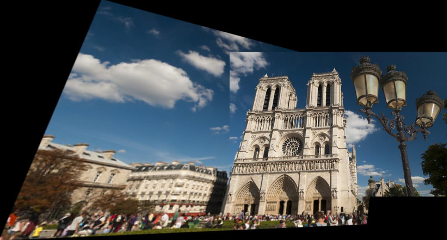
Homography is a type of transformation that links two different images, mapping points from one image to another. Think of it as a way to transform one image plane into another, making the two images align with each other, even if they were taken from different angles.

After applying the homography transformation, the first image aligns with the second one, as shown below.

There are two types of image transformations:

• Affine Transforamtion
• Projective Transformation (also known as Homography, shown above)

Affine Transformations

Affine transformations are simpler than homography. They involve:

• Translation: Moving an image from one place to another.
• Scaling: Making the image bigger or smaller.
• Rotation: Turning the image around a point.
• Shearing: Skewing the image like a parallelogram.

Properties of Affine Transformations:

• Lines stay as lines: Straight edges in the image will remain straight.
• Parallel lines stay parallel: If two lines are parallel in the original image, they'll still be parallel after transformation.
• Ratios are preserved: The relative size of objects in the image remains the same.
• Closed under composition: Applying multiple affine transformations one after another still results in an affine transformation.

Transforming a square

Lets try to understand image transformation by transforming a square. Define a set of points representing the corners of a square with the following coordinates: (-1, -1), (1, -1), (1, 1), (-1, 1), and back to (-1, -1) to close the square.

# Define the corners of a square and make them homogeneous coordinates
original_pts = np.array([[-1, -1], [1, -1], [1, 1], [-1, 1], [-1, -1]]).T
# Add a row of ones to convert the points to homogeneous coordinates
original_pts = np.vstack((original_pts, np.ones(square_corners.shape[1])))

Here, we define a set of points that represent a square shape. The np.array function creates a NumPy array containing the x and y coordinates of each corner in a counter-clockwise order. We have represented these points using homogeneous coordinates, which means we have added an extra dimension (a third coordinate, typically set to 1) to each point. This allows for more flexible transformations, such as translations, which cannot be easily handled with standard Cartesian coordinates. Lets visualize it.

plt.plot(original_pts[0,:], original_pts[1,:], label='Original Square', color='blue')

Scaling transforms the points using the equations $x' = ax$ and $y' = by$. When $a$ and $b$ are greater than 1, the square enlarges; when they are less than 1, it shrinks. If $a$ and $b$ differ, the aspect ratio of the square changes. In matrix form, this transformation is represented as:

$$\begin{equation*} \begin{bmatrix} x' \\ y' \\ 1 \end{bmatrix} = \begin{bmatrix} a & 0 & 0 \\ 0 & b & 0 \\ 0 & 0 & 1 \end{bmatrix} \begin{bmatrix} x \\ y \\ 1 \end{bmatrix} \end{equation*}$$

Rotation involves rotating the image around a fixed point, typically the origin or the image's center. The rotation matrix for a 2D transformation is given by:

$$R(\theta) = \begin{bmatrix} \cos \theta & -\sin \theta & 0 \\ \sin \theta & \cos \theta & 0 \\ 0 & 0 & 1 \end{bmatrix}$$

where $\theta$ is the angle of rotation. When applied to a point $(x, y, 1)$, this matrix rotates the point by $\theta$ degrees around the origin.

Translation involves shifting the points by a specific distance along the x and y axes, without altering its orientation or shape. In 2D, the translation operation can be represented using a matrix as follows:

$$T(dx, dy) = \begin{bmatrix} 1 & 0 & dx \\ 0 & 1 & dy \\ 0 & 0 & 1 \end{bmatrix}$$

Where $dx$ and $dy$ are the distances to shift the image in the $x$ and $y$ directions, respectively. The translation matrix moves each point in the image by adding $dx$ to the x-coordinate and $dy$ to the y-coordinate.

Shear is a transformation that distorts the shape of an image by shifting its pixels in one direction while keeping the other direction fixed. Unlike rotation or translation, shear changes the angles between lines in the image, making it a non-uniform transformation. In 2D, shear can be applied either along the x-axis, the y-axis, or both.

The shear matrix for 2D transformations is defined as:

$$S_x(s_x) = \begin{bmatrix} 1 & s_x & 0 \\ s_y & 1 & 0 \\ 0 & 0 & 1 \end{bmatrix}$$

Where $s_x$ is the shear factor along the x-axis, and $s_y$ is the shear factor along the y-axis. Shearing causes the image to be stretched or compressed along a particular axis, distorting its straight lines into slanted shapes. While shear can be useful for effects like skewing or simulating perspective, it also alters the overall geometry and proportions of the image.

Affine Transformation is any combination of scale, rotation, translations and shear. An affine transformation can be represented by the following matrix:

$$A = \begin{bmatrix} a_{11} & a_{12} & t_x \\ a_{21} & a_{22} & t_y \\ 0 & 0 & 1 \end{bmatrix}$$

Where:

• $a_{11}, a_{12}, a_{21}, a_{22}$ are the coefficients that define linear transformations (such as rotation, scaling, or shearing).
• $t_x$ and $t_y$ represent the translation (shifting) along the x and y axes, respectively.

When applied to an image, an affine transformation takes each point $(x, y)$ in the image, applies the linear transformation using the matrix $A$, and then applies the translation. The general formula for an affine transformation in homogeneous coordinates is:

$$\begin{bmatrix} x' \\ y' \\ 1 \end{bmatrix} = \begin{bmatrix} a_{11} & a_{12} & t_x \\ a_{21} & a_{22} & t_y \\ 0 & 0 & 1 \end{bmatrix} \begin{bmatrix} x \\ y \\ 1 \end{bmatrix}$$

Lets see the affine transformation in action

scale_factor = 1
rotation_angle = 0  # in degrees
shear_factor = .1

These variables define the values for scaling, rotation, and shearing.

• scale_factor: This controls the size of the transformed shape. A value greater than 1 will enlarge the square, while a value less than 1 will shrink it.
• rotation_angle: This specifies the rotation angle in degrees. A positive value rotates clockwise, and a negative value rotates counter-clockwise.
• shear_factor: This defines the amount of shearing applied to the shape. A positive value will skew the square to the right, and a negative value will skew it to the left.

Create Transformation Matrices:

scale_matrix = np.array([[scale_factor, 0, 0],
                          [0, scale_factor, 0],
                          [0, 0, 1]])

rotation_angle_rad = np.radians(rotation_angle)
rotation_matrix = np.array([[np.cos(rotation_angle_rad), -np.sin(rotation_angle_rad), 0],
                             [np.sin(rotation_angle_rad), np.cos(rotation_angle_rad), 0],
                             [0, 0, 1]])

shear_matrix = np.array([[1, shear_factor, 0],
                          [shear_factor, 1, 0],
                          [0, 0, 1]])

Here, we create individual NumPy arrays for each transformation:

• scale_matrix: This matrix scales the object uniformly based on the scale_factor.
• rotation_matrix: This matrix rotates the object by the specified rotation_angle in radians (converted from degrees using np.radians).
• shear_matrix: This matrix applies a shearing effect based on the shear_factor.

Combine Transformations:

affine_matrix = np.dot(shear_matrix, np.dot(rotation_matrix, scale_matrix))

This line combines the individual transformation matrices using matrix multiplication with np.dot. The order of multiplication matters, as it determines the order in which the transformations are applied. Here, we perform shearing, then rotation, and finally scaling.

Apply Transformation to Points

transformed_pts = np.dot(affine_matrix, original_pts)

Here, we apply the combined affine_matrix to the original points (original_pts) using matrix multiplication. This results in a new set of points representing the transformed square.

Visualize the Transformed Square:

plt.plot(transformed_pts[0,:], transformed_pts[1,:], label='Transformed Square', linestyle='dashed', color='red')

To apply the same transformation matrix used for altering the square to an entire image, we will utilize the warpPerspective function. This function allows us to perform a perspective transformation on the image, effectively applying the combined affine transformations of scaling, rotation, and shearing. The process is as follows:

T_matrix = np.array([[1, 0, image.shape[1]/2],
                     [0, 1, image.shape[0]/2],
                     [0, 0, 1]])
affine_matrix = np.dot(np.dot(T_matrix, affine_matrix), np.linalg.inv(T_matrix))
output_image = cv2.warpPerspective(image, affine_matrix, (image.shape[1], image.shape[0]))

In the given code, T_matrix is used to apply a centering transformation around the image before performing the affine transformation, and then to reverse that centering after the transformation. The purpose of this approach is to ensure that transformations like rotations, scalings, or skews happen around the center of the image, rather than around the origin (which is the top-left corner of the image in the default coordinate system).

---

Projective Transformations

Projective transformations are a more complex version of affine transformations. They combine affine transformations with additional warping (like when an object looks distorted because it's being viewed from an angle). Projective Transformations are also called Homography.

Properties of Projective Transformations:

• Lines stay as lines: Like affine, straight edges remain straight.
• Parallel lines don't always stay parallel: Unlike affine, lines that are parallel may no longer be parallel after the transformation (imagine how railroad tracks look like they converge in the distance).
• Ratios are not preserved: The relative size of objects may change.
• Closed under composition: Like affine transformations, applying multiple projective transformations results in a new projective transformation.
• A projective transformation is represented by a 3x3 matrix, which looks like this:

$$\begin{pmatrix} a & b & c \\ d & e & f \\ g & h & 1 \end{pmatrix}$$

• The parameters $g$ and $h$ in the projective transformation matrix are responsible for encoding the perspective distortion effects.
• Projective matrix has 8 degrees of freedom (DOF):
• These 8 parameters give the projective transformation 8 degrees of freedom (DOF). They allow the transformation to handle translation, rotation, scaling, shearing, and perspective distortion (how objects appear smaller in the distance).

In summary, while affine transformations handle basic transformations (like resizing, rotating, and shifting), projective transformations can deal with more complex changes in perspective, like when an object appears stretched or compressed based on the viewer's angle.

Applying Perspective Transformation (Homography) to a Checkerboard Pattern

Let's explore how modifying the parameters $g$ and $h$ in the projective transformation matrix affects the application of the perspective transform. These parameters are crucial as they introduce perspective distortion, altering how the image is perceived, especially in terms of depth and angle. By adjusting $g$ and $h$, we can simulate the effect of viewing the image from different perspectives, which can make objects appear closer or further away, or skewed in various directions. This exploration will help us understand the flexibility and power of projective transformations in computer vision.

Image Rectification

You’ve probably used or seen scan apps that can automatically straighten and correct the perspective of a document, even if it was captured from a slight angle. These apps perform image rectification, making the document appear as if it were taken perfectly from above, removing any skew caused by the angle of the camera. In this section, we'll dive into how this is done using homography transformation. We'll walk through how homography allows us to map the distorted image of a paper onto a plane, effectively "rectifying" it, so it appears as though it was captured directly from the front. This technique is a powerful tool in computer vision and image processing, and you'll see how it can be applied to real-world scenarios like document scanning or even correcting images taken in less-than-ideal conditions.

We will begin by loading the image, where the document is visible at an angle. In real applications, the corners of the document are typically detected automatically, but for this example, we will manually specify the four corner points. Next, we map these points to the corresponding corners of an A4 sheet of paper. Using OpenCV's cv2.getPerspectiveTransform, we calculate the homography matrix that transforms the document's corners to align with the A4 paper. Finally, we apply the transformation with cv2.warpPerspective to rectify the image and remove the perspective distortion.

# Load the image
image = cv2.imread('<image path>')

# Four corners of the document
pts = [(269, 187),  # top-left
       (915, 161),  # top-right
       (73, 920),   # bottom-left
       (1107, 939)] # bottom-right

input_pts = np.array(pts, dtype=np.float32)

# A4 paper dimensions
width = 400
height = int(1.41 * width) 
output_pts = np.array([(0, 0), 
                       (width-1, 0),
                       (0, height-1),
                       (width-1,height-1)], np.float32)

# compute the homography matrix
H = cv2.getPerspectiveTransform(input_pts, output_pts)

# Apply Transformation
output_image = cv2.warpPerspective(image, H, (width, height), flags=cv2.INTER_LINEAR)

Conclusion

In this blog, we've explored image transformations in computer vision, focusing on both affine and projective transformations. Affine transformations, such as translation, scaling, rotation, and shearing, offer simpler geometric manipulations that preserve lines and parallelism but may distort the overall shape. Projective transformations, on the other hand, allow for more complex operations, including perspective distortion, making them essential in tasks such as image stitching and panorama generation.

---

FAQs

What are affine transformations? Answer: Affine transformations are geometric operations that preserve points, straight lines, and planes. They include translation, scaling, rotation, and shearing. These transformations maintain the parallelism of lines and the ratios of distances between points, but they do not preserve angles or lengths in general.

How does a projective transformation differ from an affine transformation? Answer: Projective transformations (also known as homographies) are more complex than affine transformations. They can introduce perspective distortion, which makes parallel lines appear to converge. Unlike affine transformations, projective transformations do not preserve the relative size of objects or the parallelism of lines in general.

What is homography, and how is it used in image transformations? Answer: Homography is a type of projective transformation that relates two different images of the same scene, mapping points from one image plane to another. It is particularly useful in tasks like image stitching and panorama creation, where multiple views of a scene are aligned.

How do I apply affine transformations to an image? Answer: To apply affine transformations to an image, you use a transformation matrix that includes operations like scaling, rotation, translation, and shearing. These transformations can be performed using libraries like OpenCV or NumPy in Python, using functions like cv2.warpAffine().

What is the difference between affine and projective transformations in terms of real-world applications? Answer: Affine transformations are used for simpler, linear transformations where object shapes and proportions remain consistent, such as resizing, rotating, and translating an image. Projective transformations are used in more complex scenarios like 3D to 2D perspective projection, aligning images taken from different viewpoints, or creating panoramas.

Why are affine transformations important in computer vision? Answer: Affine transformations are fundamental in many computer vision tasks such as object detection, image registration, and tracking. They are used to normalize images, making them invariant to changes in position, size, and orientation, which helps in recognizing objects from different perspectives.

What are homogeneous coordinates and why are they used in transformations? Answer: Homogeneous coordinates are a system that extends Cartesian coordinates by adding an extra dimension, enabling more complex transformations like translation. They allow for the representation of points and transformations in a unified matrix form, making operations like affine and projective transformations easier to implement.

What role do projective transformations play in image stitching? Answer: Projective transformations (homographies) are essential in image stitching. When images are captured from different angles, homography can be used to align them based on common points, helping to create a seamless panorama or a single unified image.

How can I visualize affine and projective transformations in Python? Answer: You can visualize affine and projective transformations using libraries like NumPy, OpenCV, and Matplotlib in Python. By applying transformation matrices to points or images and plotting the results, you can observe how the shapes change under different transformations.

Can affine transformations be used to correct perspective distortions in images? Answer: No, affine transformations cannot correct perspective distortions because they do not account for vanishing points or depth. To correct perspective distortions, projective transformations (homographies) must be applied as they handle more complex perspective changes.