Seeing the Unseen: Unveiling Edges in Images with Edge Detection

The human eye is a marvel of perception, effortlessly gleaning shapes and objects from a visual scene. But how do computers achieve this feat? One crucial step in computer vision is edge detection.

It involves identifying significant changes in intensity within an image, which often correspond to boundaries of objects or features of interest. These edges carry most of the semantic and shape information from the image, making them crucial for understanding and analyzing visual data.

What are Edges?

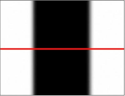
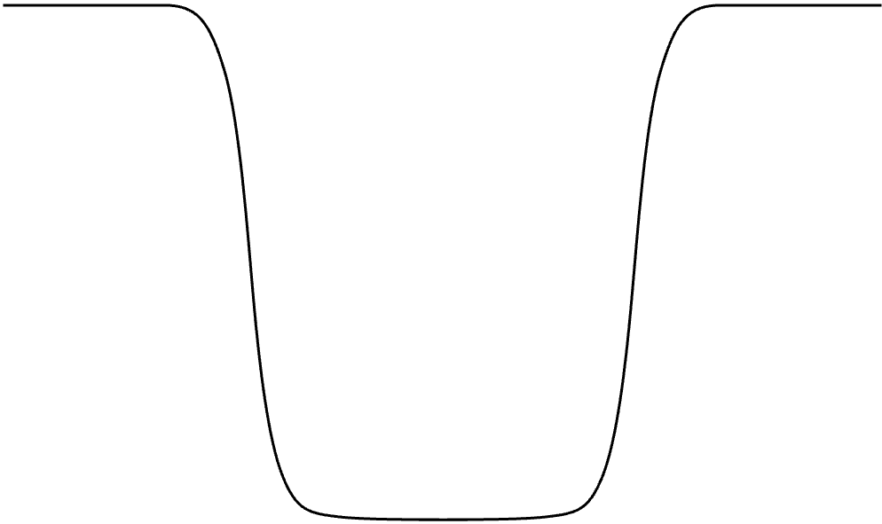
Imagine an image with varying brightness levels. An edge occurs where there is a sharp transition from light to dark or vice versa. As shown in the image, the intensity levels along the red scan line vary in brightness across the image width

An edge is a point in the image where the intensity function undergoes a rapid change. Mathematically, edges can be detected using derivatives. For a 2D function $f(x,y)$ the partial derivative with respect to $x$ is given by::

\frac{\partial f(x,y)}{\partial x} = f(x+1,y)-f(x,y)

As the animation below illustrates, the derivative is non-zero near the edges and the magnitude of the gradient reflects the intensity of the change.

To detect edges along both the $x$ and $y$ axes, we use the following:

\nabla f = \left( \dfrac{\partial f}{\partial x}, \dfrac{\partial f}{\partial y} \right)

Here, $\nabla f$ represents the gradient of the image. The gradient represents the rate of change in intensity along the $x$ -axis and $y$ -axis. The magnitude of the gradient reflects the intensity of the change, while its direction tells us where the change is happening (horizontal, vertical, or diagonal). These derivatives can be implemented as convolution operations using specific filters or kernels.

Convolution Implementation

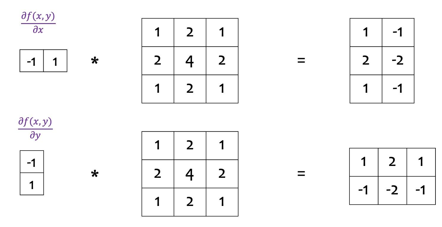
Convolution is a core operation in many low-level computer vision tasks. For example we can use the following one dimensional filters to find the partial derivates w.r.t $x$ and $y$ directions.

implementing the derivative using convolution

Sobel Operator

The Sobel operator, for example, is a popular choice for edge detection. Its $3x3$ filter as oppose to the 1D filter defined above. It calculates the gradient of the image intensity, highlighting regions with high spatial frequency which correspond to edges.

It uses two convolution kernels:

Horizontal Gradient (Sobel-X Kernel):

G_x = \begin{bmatrix} -1 & 0 & 1 \\ -2 & 0 & 2 \\ -1 & 0 & 1 \end{bmatrix}

This kernel detects edges in the vertical direction.

Vertical Gradient (Sobel-Y Kernel):

G_y = \begin{bmatrix} -1 & -2 & -1 \\ 0 & 0 & 0 \\ 1 & 2 & 1 \end{bmatrix}

This kernel detects edges in the horizontal direction.

Applying Sobel Filters

To find the gradient of an image using these kernels:

Convolve the Image with the Horizontal Kernel:

This calculates the partial derivative with respect to $x$ , giving the horizontal changes in intensity.
```
edges_x = cv2.filter2D(image, cv2.CV_32F, kernel_x)
```
Convolve the Image with the Vertical Kernel:

This calculates the partial derivative with respect to $y$ , giving the vertical changes in intensity.
```
edges_y = cv2.filter2D(image, cv2.CV_32F, kernel_y)
```

Calculating Gradient Magnitude and Direction

After computing the gradients:

Gradient Magnitude:

The gradient magnitude combines both horizontal and vertical gradients to measure the strength of edges.
$\|\nabla f\| = \sqrt{\left(\frac{\partial f}{\partial x}\right)^2 + \left(\frac{\partial f}{\partial y}\right)^2}$
```
magnitude = np.sqrt(edges_x**2 + edges_y**2)
```
Gradient Direction:

The direction of the gradient indicates the orientation of the edge.
$\theta = \tan^{-1}\left(\frac{\frac{\partial f}{\partial y}}{\frac{\partial f}{\partial x}}\right)$
```
direction = np.arctan2(edges_y, edges_x)
```

Finding Noisy Edges

To effectively find edges in an image and reduce the impact of noise, the common approach involves two main steps: smoothing the image and then applying edge detection. The goal of smoothing is to reduce noise and minor variations in the image that could interfere with accurate edge detection. This is typically done using a Gaussian filter, which blurs the image and helps in removing high-frequency noise.

import cv2
# Read the image
image = cv2.imread('path/to/image.jpg', cv2.IMREAD_GRAYSCALE)
# Apply Gaussian smoothing
smoothed_image = cv2.GaussianBlur(image, (5, 5), 1.0)

Afterwards the edges are computed using the smoothed_image

Canny Edge Detector

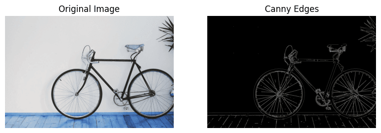
The Canny edge detector is one of the most popular methods for find the edges in an image. It involves several steps:

Smooth the image: Compute the smoothed image using Gaussian filter.

Gradient Calculation: Compute the gradient magnitude and direction using convolution with Sobel operators. This step highlights areas where intensity changes rapidly.

Non-Maximum Suppression: Thin out the edges by suppressing all gradient values that are not local maxima. This step helps to create a single-pixel wide edge line.

Thresholding: Apply a double threshold to classify edge pixels into strong, weak, or non-edges. Strong edges are retained, weak edges are considered based on their connectivity to strong edges, and non-edges are discarded.

Edge Tracking: Connect weak edges to strong edges to finalize the edges.

# Read the image
image = cv2.imread('<path to image>')
# Apply the Canny edge detector
edges = cv2.Canny(image, 150, 250)
# Display the original image and the edges side by side
plt.figure(figsize=(20, 10))
plt.subplot(141), plt.imshow(image, cmap='gray')
plt.title('Original Image'), plt.axis('off')
plt.subplot(142), plt.imshow(edges, cmap='gray')
plt.title('Canny Edges'), plt.axis('off')