Exploring Linear and Non-linear Image Filters with Python

Image filtering refers to the process of enhancing or modifying the characteristics of an image by applying a filter (or a convolution operation)

This is done by sliding a fixed-size window (called kernel or filter) over image, starting from one corner and moving horizontally and vertically. At each position of the window, a computation is performed. This computation involves taking the element-wise product of the values in the filter and the corresponding pixels in the image, summing up these products, and placing the result at the center of the window's position. This operation is known as convolution.

Image filtering is a fundamental technique in image processing used to enhance, analyze, and transform images. Filters can remove noise, enhance features, and extract important information. There are two main categories of filters: linear and non-linear. Let's dive into some common types of filters and their applications.

Linear Filters

Linear filters operate by applying a convolution operation to an image using a linear filter. The value of each pixel in the output image is a linear combination of the values of the pixels in the input image. Let $I_{ij}$ be the pixel values and $f_{uv}$ the filter values, the output is given by (for filter size of $3x3$ ):

O_{11} = I_{11}\cdot f_{11} + I_{12}\cdot f_{12} + I_{13}\cdot f_{13} + \cdots I_{33}\cdot f_{33}

Image

Output

I(1,1)

I(1,2)

I(1,3)

I(1,4)

I(1,5)

I(2,1)

I(2,2)

I(2,3)

I(2,4)

I(2,5)

I(3,1)

I(3,2)

I(3,3)

I(3,4)

I(3,5)

I(4,1)

I(4,2)

I(4,3)

I(4,4)

I(4,5)

I(5,1)

I(5,2)

I(5,3)

I(5,4)

I(5,5)

O(1,1)

O(1,2)

O(1,3)

O(2,1)

O(2,2)

O(2,3)

O(3,1)

O(3,2)

O(2,3)

Box Filter

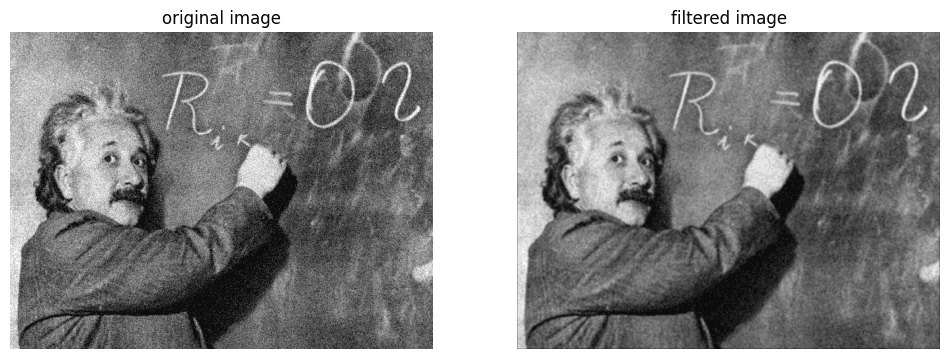
A box filter, also known as an average filter, smooths an image by averaging the pixel values within a rectangular neighborhood around each pixel. This filter is useful for reducing noise but can also blur edges. Example: For a 3x3 Box filter:

1/9 * [1 1 1
       1 1 1
       1 1 1]

import cv2
from matplotlib import pyplot as plt 
import numpy as np

# Read the image
image = cv2.imread('<path to image file>', cv2.IMREAD_GRAYSCALE)
image = gaussian_noise(image, mean = 5, sigma=25) # adding noise

# Define a 3x3 filter or kernel 
f1 = 1/9 * np.array([[1,1,1],
                     [1,1,1],
                     [1,1,1]])

# Apply the kernel using convolution
output = cv2.filter2D(src=image, ddepth=cv2.CV_32F, kernel=f1, borderType=cv2.BORDER_CONSTANT)
# Display the original and filtered image
plt.figure(figsize=(12,10))
plt.subplot(121)
plt.imshow(image, cmap = 'gray')
plt.title('Original Image'), plt.axis('off')

plt.subplot(122)
plt.imshow(output, cmap = 'gray')
plt.title('Filtering Image'), plt.axis('off')

OpenCV cv2.boxFilter can also be used to apply the box filter.

Gaussian Filter

A Gaussian filter is a type of linear filter that uses a Gaussian function to weigh the pixel values. It provides a smooth, natural blur and preserves edges better than a box filter. Example: For a 3x3 Gaussian filter with σ = 1:

1/16 * [1 2 1
        2 4 2
        1 2 1]

# Read the image
image = cv2.imread('<path>', cv2.IMREAD_GRAYSCALE)

# Apply the box filter
box_filtered_image = cv2.boxFilter(image, -1, ksize=(7,7), borderType=cv2.BORDER_CONSTANT)
# Apply Gaussian filter
gaussian_filtered_image = cv2.GaussianBlur(image, ksize=(7,7), sigmaX = 3, sigmaY = 3, borderType=cv2.BORDER_CONSTANT)

# Display the original and smooth filter
plt.figure(figsize=(12, 10))

plt.subplot(1, 3, 1)
plt.imshow(cv2.cvtColor(image[200:300,200:300], cv2.COLOR_BGR2RGB))
plt.title('Original Image')
plt.axis('off')

plt.subplot(1, 3, 2)
plt.imshow(cv2.cvtColor(box_filtered_image[200:300,200:300], cv2.COLOR_BGR2RGB))
plt.title('Box Filtered Image')
plt.axis('off')

plt.subplot(1, 3, 3)
plt.imshow(cv2.cvtColor(gaussian_filtered_image[200:300,200:300], cv2.COLOR_BGR2RGB))
plt.title('Gaussian Filtered Image')
plt.axis('off')

Non-linear Filters

In the context of computer vision, non-linear filters are image processing techniques used to manipulate or enhance images in ways that linear filters cannot. Unlike linear filters, which apply a linear transformation to the input image, non-linear filters use more complex operations that often involve sorting, ranking, or non-linear functions. These filters are particularly useful for tasks such as noise reduction, edge detection, and image enhancement.

Median Filter

The median filter is one of the most widely used non-linear filters. The median filter replaces each pixel value with the median value of its neighbors within a specified kernel. It is highly effective in removing salt-and-pepper noise while preserving edges.

Example: For a 3x3 kernel, if the neighborhood pixel values are [2, 3, 8, 4, 5, 1, 7, 9, 6], the median filter will first sort the pixel values: [1,2,3,4,5,6,7,8,9]. Then it finds the median which is 5.

# Read the image
image = cv2.imread('<path>', cv2.IMREAD_GRAYSCALE)
# Add noise
image = sp_noise(image, .1)
# Define the size of the box filter kernel (e.g., 3x3)
kernel_size = (6, 6)
# Apply the Gaussian and median filter
gaussian_filtered_image = cv2.GaussianBlur(image, ksize=(5,5), sigmaX = 2, sigmaY = 2, borderType=cv2.BORDER_CONSTANT)
median_filtered_image = cv2.medianBlur(image, ksize=5)

# Display the original and smooth filter
plt.figure(figsize=(12, 10))

plt.subplot(1, 3, 1)
plt.imshow(cv2.cvtColor(image, cv2.COLOR_BGR2RGB))
plt.title('Original Image')
plt.axis('off')

plt.subplot(1, 3, 2)
plt.imshow(cv2.cvtColor(gaussian_filtered_image, cv2.COLOR_BGR2RGB))
plt.title('Gaussian Filtered Image')
plt.axis('off')

plt.subplot(1, 3, 3)
plt.imshow(cv2.cvtColor(median_filtered_image, cv2.COLOR_BGR2RGB))
plt.title('Median Filtered Image')
plt.axis('off')

Padding

Padding is a technique to handle the boundary regions of data.

Zero Pad (Zero-padding): Add zeros around the boundary of the input data to ensure complete coverage in convolutional operations.

Wrap Around (Circular Padding): Treat the data as if it were wrapped around, creating a circular effect, suitable for periodic or circularly continuous data.

Copy Edge (Replication Padding or Extend): Replicate the edge values of the input to maintain spatial dimensions and ensure consistency with nearest input values.

Reflect Across Edge (Reflective Padding or Mirror Padding): Reflect the input values across the edges to reduce artifacts and provide a smoother transition at the boundaries.

Conclusion

Image filtering is an essential technique in image processing, with various filters suited to different tasks. Linear filters like the box and Gaussian filters are excellent for general smoothing, while non-linear filters like the median filter are superior for noise removal and edge preservation. Understanding and choosing the right filter can significantly enhance the quality and analysis of images in various applications.