The science of image formation and color

Image formation is the process by which a scene is captured and represented as an image, typically by a camera or another imaging device. This process involves several key steps:

Light Interaction: Light from a scene interacts with objects, reflecting and refracting based on the objects' properties.
Capture: A camera lens focuses the light onto a sensor, which converts the light into an electrical signal.
Conversion: The electrical signal is then processed and converted into a digital image.

The quality of the image depends on various factors, including the camera's resolution, sensor technology, and color-capturing capabilities. An image can be represented as a matrix of pixel values, where each value corresponds to the amount of light at that specific point. The value of a pixel in this matrix can typically range from 0 to 255, fitting in a byte (uint8), or from 0 to 1, represented as a floating point number (float32). Addressing pixels is done by specifying their coordinates as (i, j), where 'i' represents the row and 'j' represents the column. The coordinate (0, 0) refers to the top-left pixel. In a 3-dimensional array (3-channel image), each pixel is represented by three values corresponding to the intensities of the red, green, and blue colors.

# Reading and image and displaying using OpenCV Python library
import cv2
# Read the image from a file
image = cv2.imread('path_to_image.jpg')
# Check if the image was successfully loaded
if image is None:
    print("Error: Could not open or find the image.")
else:
    # Display the image in a window
    cv2.imshow('Image', image)
    # Wait for a key press indefinitely or for a specified amount of time in milliseconds
    cv2.waitKey(0)
    # Destroy all the window we created
    cv2.destroyAllWindows()

What is Color?

Color perception arises from how our eyes and brain interpret the various wavelengths of light. Visible light spans from about 400 nm (violet) to 700 nm (red), and the colors we see are determined by how these wavelengths interact with photoreceptor cells in our eyes. These cells, found in the retina, include rods, which are highly sensitive to light but do not detect color, and cones, which are less sensitive but crucial for color vision in bright light. There are three types of cone cells, each responding to different wavelengths: blue (440 nm), green (530 nm), and red (560 nm). This trichromatic system allows us to perceive a wide range of colors through combinations of these primary hues. The trichromatic theory of color, proposed by Thomas Young in the 1700s and validated through experiments like those described in Wandell's "Foundations of Vision" (Sinauer Assoc., 1995), asserts that our perception of color can be sufficiently explained by the responses of these three types of cone cells.

Source

Color Spaces

A color space is a specific organization of colors, which allows for the reproducible representation of color across different devices and media. Some common color spaces include:

RGB (Red, Green, Blue): Used in digital displays and cameras.
CMYK (Cyan, Magenta, Yellow, Black): Used in color printing.
HSV (Hue, Saturation, Value): Used in graphics design and image editing.
LAB (Lightness, A, B): Designed to be device-independent, representing human vision.

Each color space has its advantages and is chosen based on the application.

HSV Color space

HSV stands for Hue, Saturation, and Value, and it is a color space commonly used in image processing and computer vision. The HSV color space represents colors in a way that separates the chromatic information (hue and saturation) from the brightness information (value or intensity). This makes it more intuitive for humans to describe and manipulate colors.

Hue (H): Represents the type of color, such as red, green, or blue. The hue is typically represented as an angle ranging from 0 to 360 degrees in most applications. It wraps around so that 0 and 360 are the same color (red). In OpenCV hue range is [0,179]
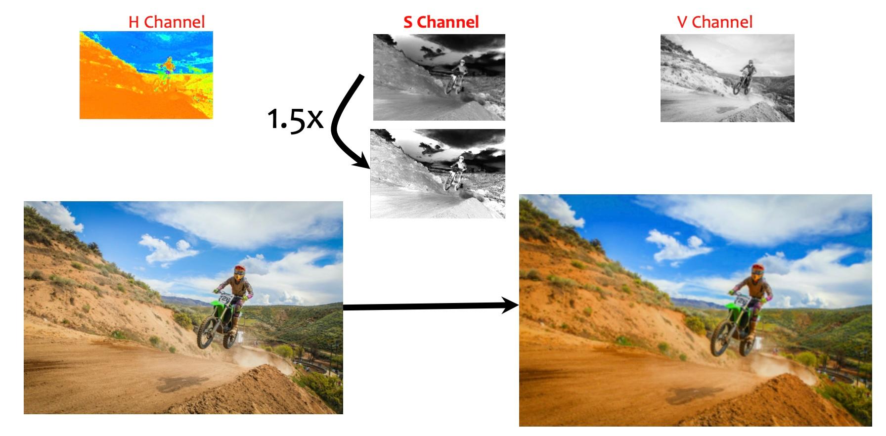
Saturation (S): Refers to the vividness or purity of the color. A saturation value of 0 corresponds to grayscale, while higher values indicate more vivid and intense colors.
Value (V) : Represents the brightness or intensity of the color. A value of 0 is black, and as the value increases, the color becomes brighter.

Increasing color saturation

Increasing color saturation using the HSV (Hue, Saturation, Value) model is about making colors more vivid without changing their basic hue (like red, green, or blue) or brightness. Saturation in HSV represents how intense or pure a color appears. By increasing saturation, you enhance the vibrancy of colors across an image. This adjustment is done by scaling up the saturation value while keeping the hue and brightness constant. The result is that colors become more lively and stand out more prominently.

# Code snippet to increase the saturation value using OpenCV
import cv2
import numpy as np
# Read the image using cv2
image = cv2.imread('path_to_image.jpg')
# Convert the image to HSV color space
image_hsv = cv2.cvtColor(image, cv2.COLOR_BGR2HSV)
# Split the HSV image into its three channels
hue_channel, saturation_channel, value_channel = cv2.split(image_hsv)
# Modify the saturation channel
modified_channel = np.clip(1.5 * saturation_channel, 0, 255).astype(np.uint8)
# Merge the modified channels back into an HSV image
modified_hsv_image = cv2.merge([hue_channel, modified_channel, value_channel])
# Convert the modified HSV image back to BGR color space
modified_image = cv2.cvtColor(modified_hsv_image, cv2.COLOR_HSV2BGR)
# Display the original and modified images side by side (if using Jupyter Notebook or similar)
cv2.imshow('Original Image', image)
cv2.imshow('Modified Image', modified_image)
cv2.waitKey(0)
cv2.destroyAllWindows()

example to show how to increase the color in an image using HSV colorspace

Histogram

A histogram is a graphical representation of the distribution of pixel intensity values in an image. It shows the frequency of each intensity value, ranging from 0 (black) to 255 (white) in an 8-bit grayscale image. Color images have separate histograms for each channel (Red, Green, and Blue).

Histograms are useful for:

Analyzing Exposure: Identifying underexposed or overexposed regions.
Enhancing Contrast: Adjusting the intensity values to improve image quality.
Thresholding: Segmenting an image based on intensity values.

# Read the image
image = cv2.imread('path_to_image.jpg', cv2.IMREAD_GRAYSCALE)
# Calculate the histogram
histSize = 256
hist = cv2.calcHist([image], [0], None, [histSize], [0, 256])

White Balancing

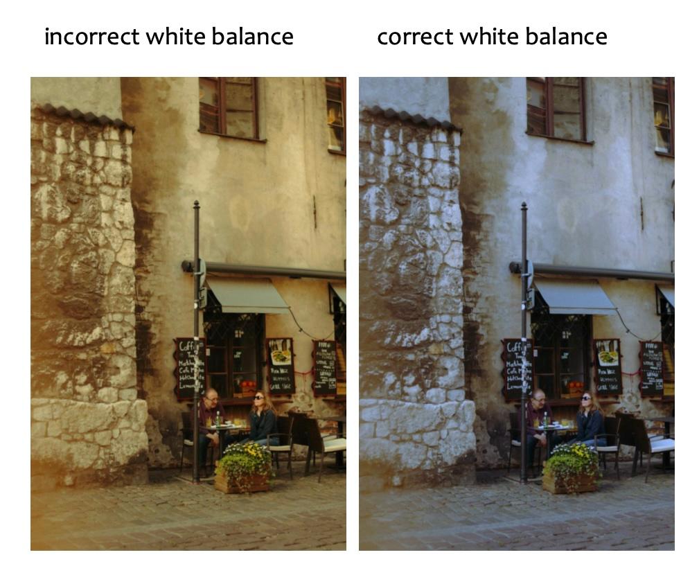
White balancing is the process of adjusting the colors in an image to ensure that the whites appear neutral (i.e., without any color cast). This is essential because different light sources have different color temperatures, which can affect the colors in an image.

Common methods for white balancing include:

Auto White Balance: The camera or software automatically adjusts the white balance.
Preset White Balance: Using predefined settings for different lighting conditions (e.g., daylight, tungsten).
Manual White Balance: Manually selecting a neutral reference point in the image.
Gray world assumption: Assume the scene is on average gray

Gray world assumption

Assume the scene is on average gray:

This means that the color channels should have equal mean values.
Compute the average color values for each color channel $avg_r,avg_g, avg_b$
Compute the overall mean

avg = \frac{avg_r,avg_g, avg_b}{3}

Scale each channel by $avg/avg_r, avg/avg_g, avg/avg_b$

import cv2
import numpy as np

# Read the image
image = cv2.imread('data/images/chair.jpg')

# Convert BGR to float32 for more accurate calculations
image_float = image.astype(np.float32)
# Calculate the average intensities for each channel
avg_b = np.mean(image_float[:, :, 0])
avg_g = np.mean(image_float[:, :, 1])
avg_r = np.mean(image_float[:, :, 2])
# Find the overall average intensity
avg_gray = (avg_b + avg_g + avg_r) / 3
# Calculate scaling factors for each channel
scale_b = avg_gray / avg_b
scale_g = avg_gray / avg_g
scale_r = avg_gray / avg_r
# Apply the scaling factors to each channel
balanced_image_float = cv2.merge([
    image_float[:, :, 0] * scale_b,
    image_float[:, :, 1] * scale_g,
    image_float[:, :, 2] * scale_r
])
# Clip the values to ensure they are within the valid range
balanced_image_float = np.clip(balanced_image_float, 0, 255)
# Convert the result back to uint8 format
balanced_image = balanced_image_float.astype(np.uint8)

Conclusion

In conclusion, understanding image formation and color is essential for various applications in computer vision. Proper use of color spaces, histograms, and white balancing techniques can significantly enhance the quality and effectiveness of images.