Local Search Algorithms: Hill Climbing, Simulated Annealing, and Genetic Algorithms

Introduction

In previous search techniques like BFS, DFS, and A*, the objective was to find a path from the start state to the goal state. However, in some scenarios, the path is irrelevant, and the primary goal is to identify the state with the highest score according to a given function. This is where local search algorithms come into play.

Local search algorithms are utilized when the path from the start to the goal is not significant. Instead, the focus is on finding the state with the optimal score. These algorithms are particularly useful in optimization problems where the aim is to discover the best state based on an objective function.

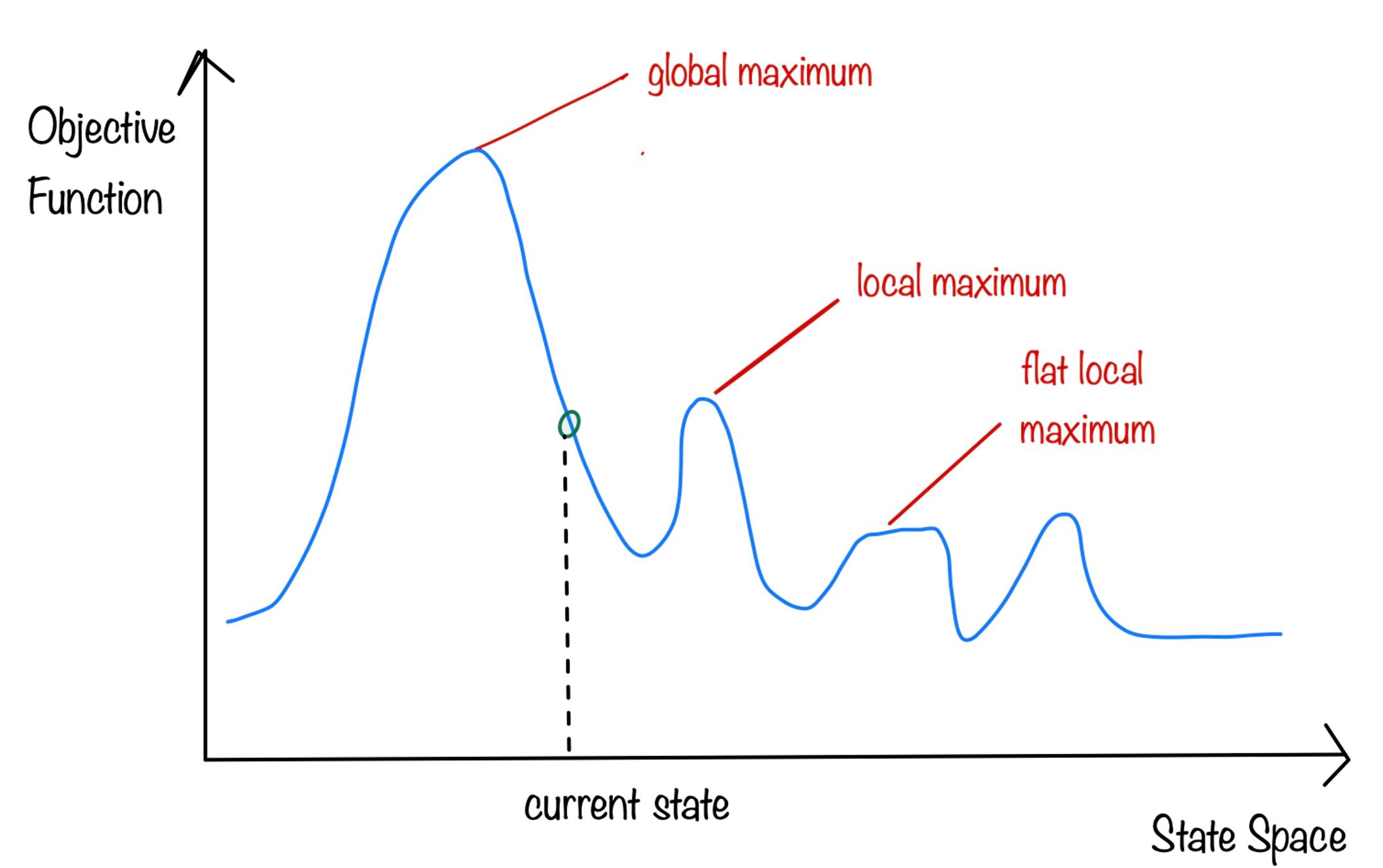
Consider the following state-space landscape where the x-axis represents the state space and the y-axis represents the value of the objective function. The goal is to identify the global maximum in this landscape. The algorithm is called Hill climbing. If the objective function is the cost then the goal is to identify the global minimum. The algorithm is call gradient descent.

In local search algorithms, each state $s$ is evaluated using a scoring function $f(s)$. The objective is to find the state with the highest score, or at least a reasonably high score, without considering the path taken to reach that state. This approach is particularly useful for optimization problems where the primary concern is the quality of the solution rather than the specific steps to achieve it. This approach can find reasonable solutions in large or infinite (continuous) state spaces for which the other algorithms are not suitable

Hill Climbing

Hill Climbing is a simple local search algorithm that starts with an arbitrary state and iteratively selects the neighboring state with the highest value. This process continues until no better neighboring state can be found. Hill Climbing is a greedy algorithm that may get stuck in local optima, as it does not consider moves to states with lower values. It keeps track of only one state at a time, moving to the best neighboring state.

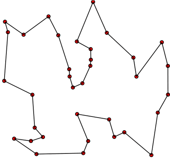
The Traveling Salesman Problem (TSP) is a classic optimization challenge where the objective is to find the shortest route that visits each city exactly once and returns to the starting point. The goal is to minimize the total distance traveled, which serves as the objective function.

To tackle this problem using Hill Climbing, we can follow these steps:

• Start with an initial random state: any random ordering of the cities (e.g., A → B → C → D → ...).
• Generate successor states by modifying the current city order (e.g., swapping two cities).
• Evaluate each state using the objective function $f$, which calculates the total length of the route.
• Select the successor state with the highest score
• Loop until no better state can be found or a stopping criterion is met.

This approach helps explore potential solutions iteratively, aiming to uncover the shortest possible route for the traveling salesman.

8-Queens Problem is another classic optimization challenge where the objective is to place eight queens on an $8\times8$ chessboard such that no two queens threaten each other. The goal is to find a configuration that satisfies this constraint. The objective function in this case calculates the number of pairs of queens threatening each other. The optimal solution has a score of 0, indicating no threats between queens.

To tackle this problem using Hill Climbing, we can follow these steps:

• Start with an initial random state: a random placement of eight queens on the chessboard, with one queen per column.
• Generate successor states by moving one queen to a different row in its column.
• Evaluate each state using the objective function $f$, which calculates the number of pairs of queens threatening each other.
• Select the successor state with the lowest score.
• Loop until no better state can be found or a stopping criterion is met.

Hill Climbing Search problems

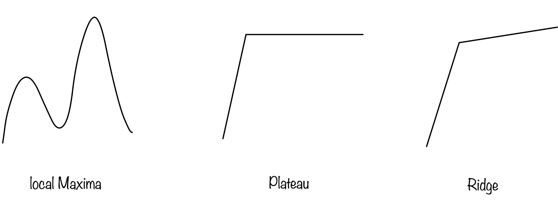
Hill Climbing is a simple and intuitive algorithm, but it has some limitations. It can get stuck in local optima, where the algorithm converges to a suboptimal solution without exploring the entire state space. This issue arises because Hill Climbing only considers moves to states with higher values, which may lead to premature convergence. The algorithm can get stuck in local maximum , plateau regions, where all neighboring states have the same value or ridges, where the path to the global maximum is narrow.

Because of these issues, the hill climbing algorithm only explores a small fraction of the state space and converges to a suboptimal solution. Variants of hill climbing algorithms have been developed to address these limitations, such as stochastic hill climbing, simulated annealing, and genetic algorithms.

Stochastic Hill Climbing

Stochastic Hill Climbing introduces randomness into the selection of neighboring states. Instead of always choosing the steepest uphill move, it randomly selects from the available uphill moves, with a probability proportional to the steepness of each move. This randomness helps the algorithm explore a broader range of the state space and potentially escape local optima.

Random Restart Hill Climbing

In random restart hill climbing, the algorithm restarts from a random initial state whenever it gets stuck in a local optima. This approach helps the algorithm explore different regions of the state space and increases the chances of finding the global maximum.

Simulated Annealing

Simulated Annealing is an optimization technique that allows for occasional moves to worse states in order to escape local optima. It simulates the annealing process in metallurgy, where a material is heated and then slowly cooled to remove defects. Heat allows atoms to escape local energy minima, moving randomly to higher-energy states. The temperature is then gradually decreased over time. Slow cooling provides atoms more opportunities to settle into configurations with lower internal energy than the starting state.

Simulated Annealing mimics this process by starting at a high "temperature," which allows for greater exploration of the solution space, including occasional moves to worse states to escape local optima. At high temperatures, the system explores broadly, enabling it to overcome barriers and avoid being trapped in suboptimal solutions. Over time, the temperature gradually decreases, reducing the likelihood of worse moves and allowing the system to stabilize in a state closer to the global optimum.

A key feature of simulated annealing is its probabilistic acceptance of worse moves, determined by the energy difference between states and the current temperature. This controlled randomness enables the algorithm to balance exploration and exploitation, making it an effective approach for solving complex optimization problems.

The following pseudocode describes the Simulated Annealing algorithm for solving optimization problems:

function SIMULATED-ANNEALING(problem, schedule) returns a solution state
    current ← problem.INITIAL
    for t = 1 to ∞ do
        T ← schedule(t)
        if T = 0 then
            return current
        next ← a randomly selected successor of current
        ∆E ← VALUE(current) – VALUE(next)
        if ∆E > 0 then
            current ← next
        else
            current ← next only with probability e^(∆E/T)

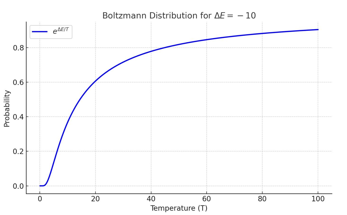
The algorithm starts with an initial state and iteratively generates successor states. If the successor state has a higher value, it is accepted as the new current state. If the successor state has a lower value, it is accepted with a probability determined by the energy difference and the current temperature. This probabilistic acceptance allows the algorithm to explore worse states and escape local optima. The temperature schedule controls the rate at which the temperature decreases over time, balancing exploration and exploitation. The algorithm terminates when the temperature reaches zero or a stopping criterion is met. The acceptance probability is determined by the Boltzmann distribution, which ensures that worse moves are accepted with a decreasing probability as the temperature decreases.

The figure below shows the Boltzmann distribution for the energy difference of $\Delta E=-10$. At high temperatures, the probability of accepting worse moves is higher, allowing for greater exploration. As the temperature decreases, the probability of accepting worse moves decreases, leading to more exploitation of better solutions.

Local Beam Search

In local beam search, multiple states are maintained in parallel, known as a "beam." The algorithm starts with multiple random states and generates successor states for each of them. The best successor states are selected to form the next generation of states. This process continues until a goal state is reached or a stopping criterion is met. Local beam search is useful for exploring multiple regions of the state space simultaneously and can help avoid getting stuck in local optima.

Local beam search is different than random restart hill climbing in that the multiple states share information and compete with each other. The best states are selected to form the next generation, allowing the algorithm to focus on promising regions of the state space. This approach can be more efficient than random restart hill climbing, as it maintains multiple states in parallel and leverages their collective knowledge to guide the search.

Genetic Algorithms

Genetic Algorithms are inspired by the process of natural selection. They work by evolving a population of states over several generations. Each state (called an individual) is evaluated based on a fitness function, and the best individuals are selected to create the next generation through crossover and mutation.

The genetic algorithm process involves the following steps:

• Initialization: Create an initial population of random individuals.
• Evaluation: Evaluate each individual using the fitness function.
• Selection: Select the best individuals to form the next generation.
• Crossover: Combine pairs of individuals to create new offspring.
• Mutation: Introduce random changes to the offspring.
• Replacement: Replace the old generation with the new generation.
• Termination: Repeat the process for a fixed number of generations or until a stopping criterion is met.

The pseudocode for the genetic algorithm is as follows:

GENETIC-ALGORITHM(population, fitness) returns an individual
repeat
    weights ← WEIGHTED-BY(population, fitness)
    population2 ← empty list
    for i = 1 to SIZE(population) do
        parent1, parent2 ← WEIGHTED-RANDOM-CHOICES(population, weights, 2)
        child ← REPRODUCE(parent1, parent2)
        if (small random probability) then
            child ← MUTATE(child)
        add child to population2
    population ← population2
until some individual is fit enough, or enough time has elapsed
return the best individual in population, according to fitness

REPRODUCE(parent1, parent2) returns an individual
n ← LENGTH(parent1)
c ← random number from 1 to n
return APPEND(SUBSTRING(parent1, 1, c), SUBSTRING(parent2, c + 1, n))

In the pseudocode above, the population is the set of individuals, and the fitness function evaluates each individual's quality. The algorithm selects parents based on their fitness, with better individuals having a higher probability of being selected. The REPRODUCE function combines the genetic material of two parents to create a new offspring. Mutation introduces random changes to the offspring, ensuring diversity in the population. The process continues for multiple generations, evolving the population towards better solutions.

Conclusion

These local search algorithms are powerful tools for solving complex optimization problems where the path to the solution is less important than the solution itself. Hill Climbing, Simulated Annealing, and Genetic Algorithms each offer unique approaches to exploring the state space and finding optimal solutions. By balancing exploration and exploitation, these algorithms can navigate complex landscapes and discover high-quality solutions efficiently.