A Beginner’s Guide to 3D Perception in Computer Vision: Structure-from-Motion Explained

Introduction

Have you ever wondered how you can judge the distance of objects around you? It's thanks to the two eyes you have, which work together to provide depth perception. If you cover one eye, it becomes much harder to estimate how far away objects are. In this blog, we will explore in detail how depth perception works, and how you can estimate the distance of objects from just two images taken from different angles. Before diving into how depth perception works from two images, let’s first discuss the fundamental camera model—the pinhole camera model.

Pinhole Camera Model

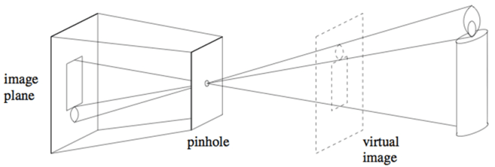
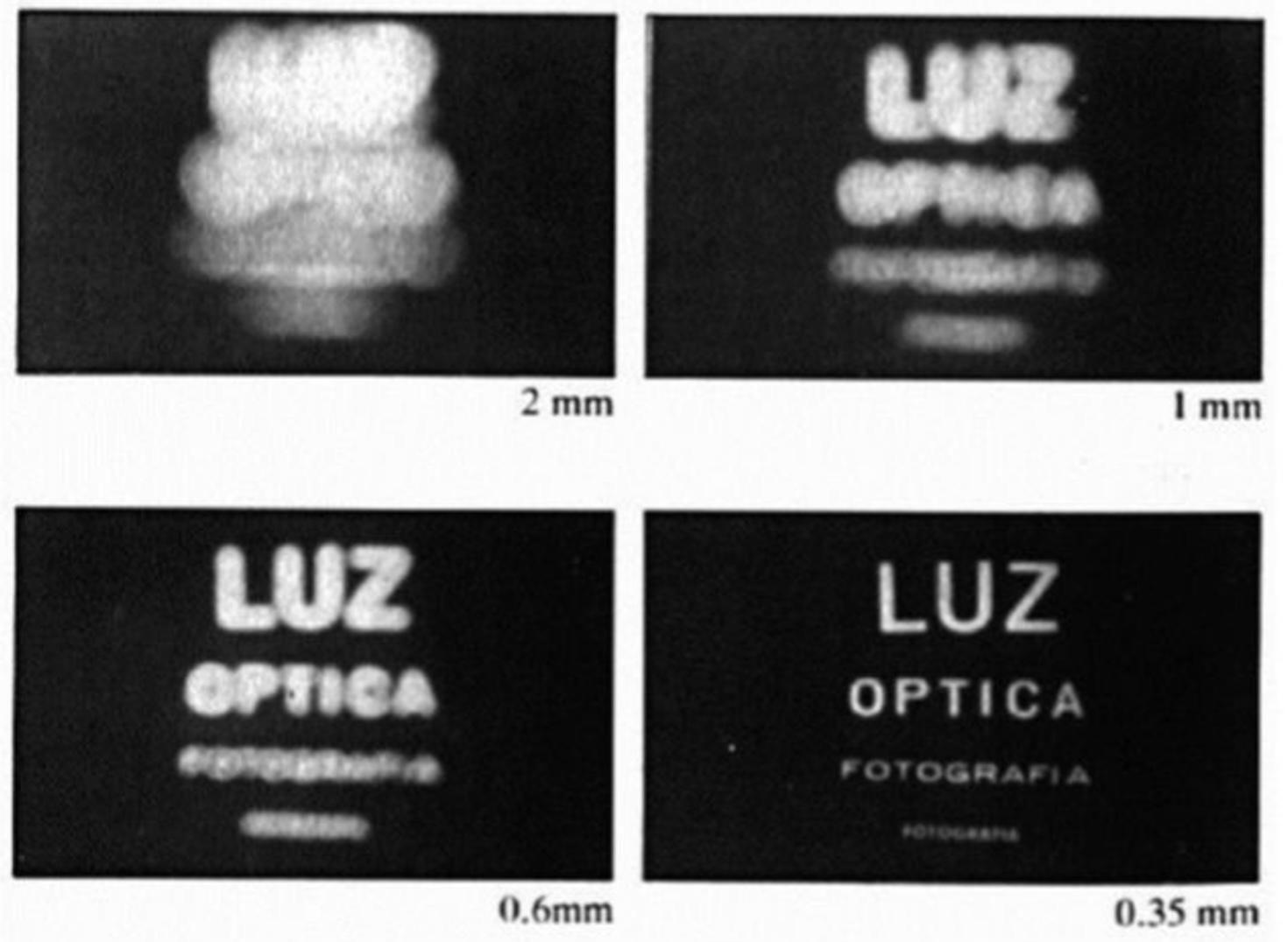
The pinhole camera model is a simplified representation of how a camera captures an image. It imagines a small hole, known as the aperture, through which light from the scene passes to form an image on a surface like film or a digital sensor. In this model, light rays entering the pinhole converge to create a virtual image. If the aperture is large, the image becomes blurred because multiple rays from the same point fall at different positions on the image plane. Conversely, a smaller aperture results in a sharper image, as the rays converge more precisely on the plane.

However, making the aperture too small reduces the brightness of the image. So, how can we increase the aperture size while maintaining focus? The solution lies in using lenses. Lenses work by bending light rays, guiding them to converge at a specific point. The degree of bending is determined by the lens's focal length, which is the distance at which the image forms. The focal length is one of the intrinsic parameters of a camera, along with other factors such as lens distortion, since each lens introduces unique distortions in the image.

Let us write the equation for how a 3D point is projected onto the image plane in a pinhole camera. The projection of a 3D point is influenced by the intrinsic parameters, such as the focal length, and the extrinsic parameters, which define the pose of the camera. Suppose the camera is rotated using a rotation matrix $R$ and translated using a translation vector $T$ with respect to the world coordinates. The projection of a 3D point $X$ on to the image place is given by the following equation:

$$x = K R (X - T)$$

To represent a 3D point $X$ in homogeneous coordinates, we typically add an extra coordinate to the point, i.e we can represent it in homogeneous coordinates as:

$$X = \begin{bmatrix} x \\ y \\ z \\ 1 \end{bmatrix}$$

The extra coordinate enables the representation of projective transformations through multiplication with transformation matrices. The projection matrix $M$ can be expressed as:

$$M_{3\times 4} = K [R \,\,| -R T]_{3\times 4}$$

Where:

• $K$ is the intrinsic matrix of the camera, which includes parameters like the focal length and the principal point.
• $R$ is the rotation matrix, representing the orientation of the camera.
• $T$ is the translation vector, representing the position of the camera in the world.

The intrinsic matrix $K$ is typically defined as:

$$K = \begin{bmatrix} f_x & 0 & c_x \\ 0 & f_y & c_y \\ 0 & 0 & 1 \end{bmatrix}$$

Where:

• $f_x$ and $f_y$ are the focal lengths in terms of pixels, along the x and y axes.
• $c_x$ and $c_y$ are the coordinates of the principal point, usually at the center of the image.

The projection of a 3D point $X$, given by $x = MX$, is converted to inhomogeneous coordinates by normalizing with the third element. Specifically, we obtain $x$ and $y$ coordinates by dividing by $z$, resulting in $x/z$ and $y/z$.

Epipolar Geometry

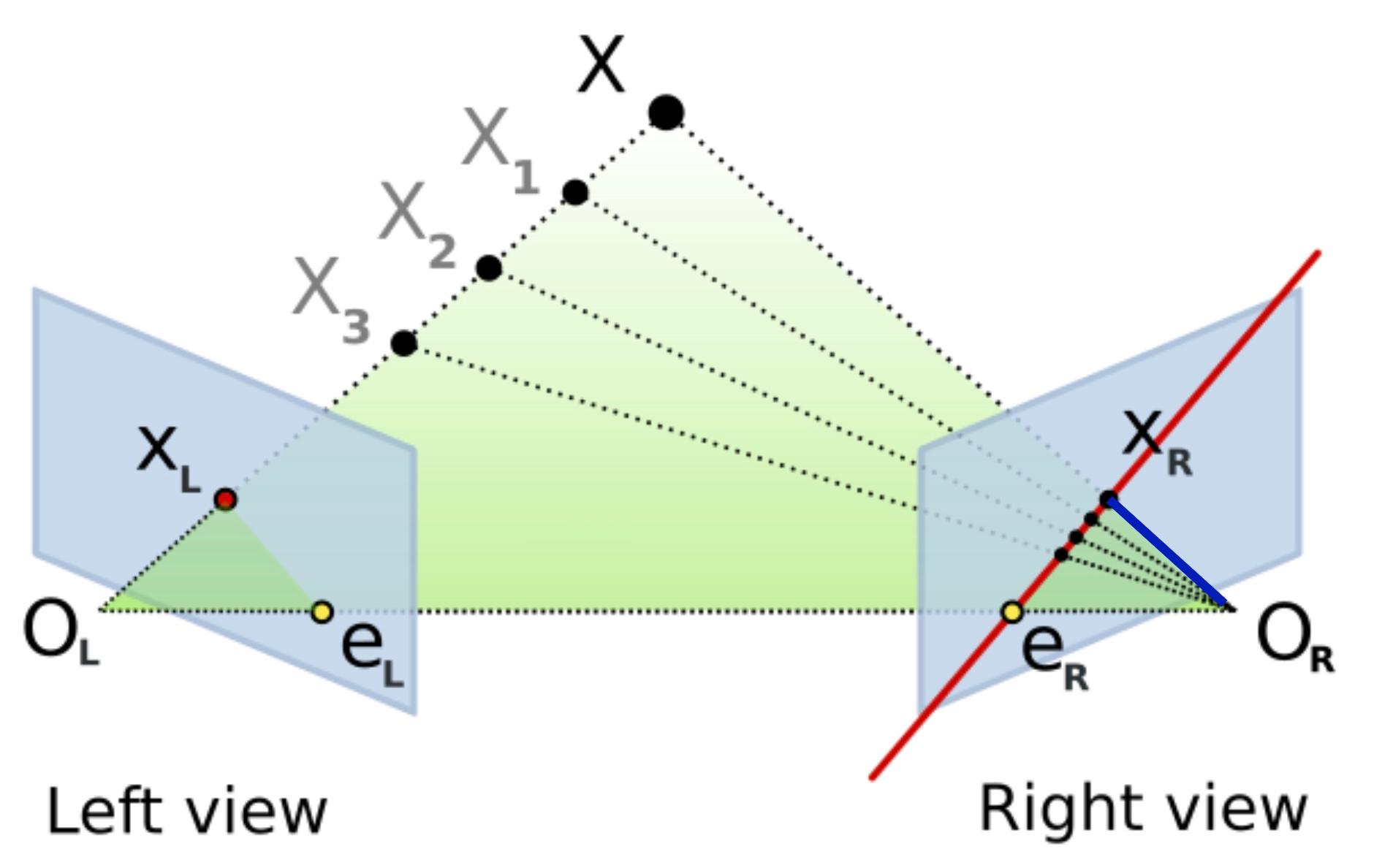
Now consider two image planes looking at the same 3D point $X$. Points $x_L$ and $x_R$ are the projections of point $X$ onto the image planes. The center of the two cameras is represented by $O_L$ and $O_R$, and the line between them is referred to as the baseline. We call the plane defined by the two camera centers and 3D point $X$ as the epipolar plane. The locations of where the baseline intersects the two image planes are known as the the epipoles $e_L$ and $e_R$. Finally, the lines defined by the intersection of the epipolar plane and the two image planes are known as the epipolar lines. The epipolar lines have the property that they intersect the baseline at the respective epipoles in the image plane.

$$l_R = E x_L$$

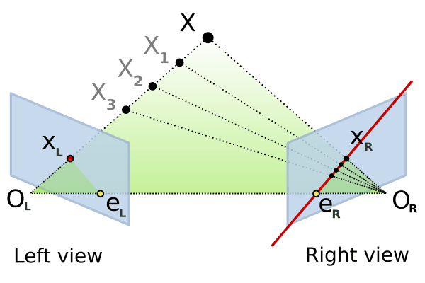
An important point to note is that all points $X_1, X_2, X_3, X$ project to the same point $x_L$ on the left image plane but project to different points on the right image plane. These projected points lie along the epipolar line in the right image (the red line in the right image plane above). This establishes a relationship between the two image planes: a single point in one image corresponds to a line in the other image. This relationship is captured by a matrix called the Essential Matrix:

$$l_R = E x_L$$

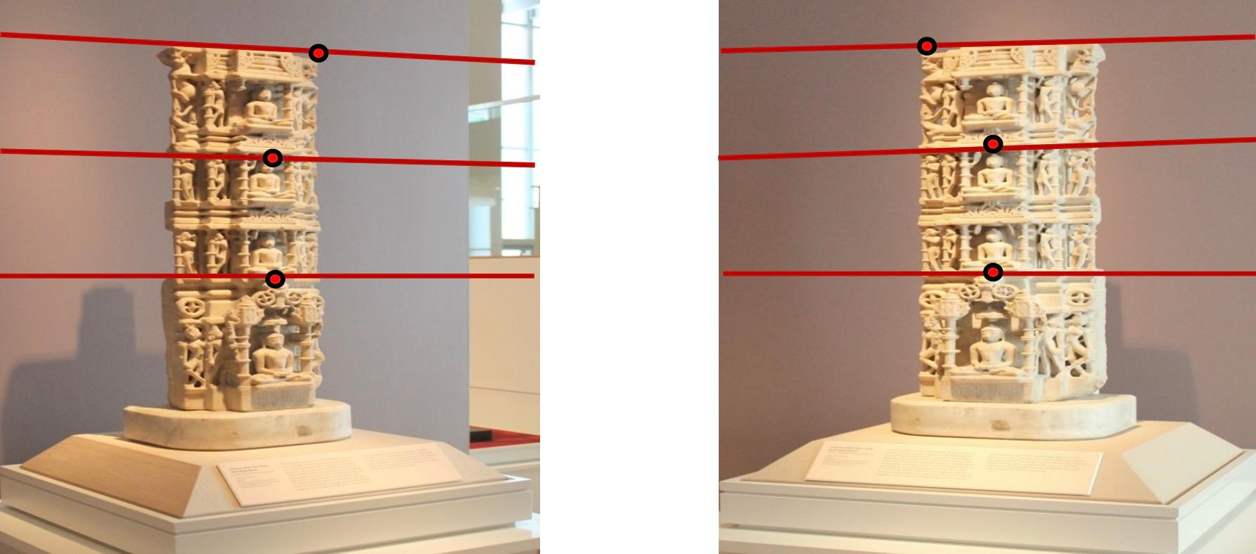
The images below illustrate the epipolar lines in both views. A point in one image corresponds to a line in the other image, a relationship defined by the Essential matrix $E$.

Essential matrix

The next question is how to determine the Essential matrix $E$ between the two images. The vectors representing the epipolar line (red line) $l_R$ and the vector (blue line) $x_R$ are orthogonal, leading to the following relationship:

$$x_R \cdot l_R = x_R^T E x_L = 0$$

The Essential matrix is a $3 \times 3$ matrix leading to 8 degrees of freedom. We need 8 corresponding points between the left and the right image to find the Essential matrix using 8-point algorithm. The Essential matrix encodes the rotation and translation of the right camera with respect to the left camera.

$$E = [T]_{\times} R$$

where $[T]_\text{x}$ is skew-symmetric matrix of translation vector $T$.

Fundamental Matrix

So far we have assumed a canonical camera - a camera with a focal length of 1 and standardized intrinsic parameters, e.g K = eye(3). In real cameras, we typically have more complex intrinsic parameters, including a specific focal length and potentially other lens distortions. The epipolar geometry is that case is described by the fundamental matrix $F$:

$$F = K_R^{-T} E K_L^{-1}$$

where $K_L, K_R$ are the intrinsic parameter matrices of the left and right camera.

Structure From Motion

Let's attempt to simulate the process described above. We'll generate 3D points to represent a cuboid using Python as follows:

import numpy as np
import cv2 as cv
import matplotlib.pyplot as plt
from mpl_toolkits.mplot3d import Axes3D

# Some helper functions
def to_homogeneous(coordinates):
    # Add a column of ones to the coordinates to make them homogeneous
    return np.hstack((coordinates, np.ones((coordinates.shape[0], 1))))
    
def from_homogeneous(coordinates):
    # Divide the first two columns by the third column to obtain non-homogeneous coordinates
    return coordinates[:, :2] / coordinates[:, 2][:, None]
# Function to plot a camera plane in 3D
def plot_camera_plane(ax, R, T, scale=0.5, color='blue', label='Camera'):
    # Define the camera plane corners in the camera's local coordinate system
    camera_corners = np.array([
        [-1, -1, 1],
        [ 1, -1, 1],
        [ 1,  1, 1],
        [-1,  1, 1],
        [-1, -1, 1]
    ]) * scale
    # Transform corners to world coordinates
    transformed_corners = (R @ camera_corners.T + T.reshape(3, 1)).T
    # Plot the camera plane as a polygon and mark the optical center
    ax.plot(*transformed_corners[:5, :].T, color=color, linestyle='-', label=label + " Plane")

# Define cuboid dimensions and center
width, height, depth = 3, 2, 2
center = np.array([0, 0, 5])
num_points = 50  # Number of points to place along each edge
# Calculate half-dimensions
w, h, d = width / 2, height / 2, depth / 2
# Define the 8 corners of the cuboid
corners = np.array([
    [center[0] - w, center[1] - h, center[2] - d],
    [center[0] + w, center[1] - h, center[2] - d],
    [center[0] + w, center[1] + h, center[2] - d],
    [center[0] - w, center[1] + h, center[2] - d],
    [center[0] - w, center[1] - h, center[2] + d],
    [center[0] + w, center[1] - h, center[2] + d],
    [center[0] + w, center[1] + h, center[2] + d],
    [center[0] - w, center[1] + h, center[2] + d]
])
# Define pairs of corners that form the edges
edges = [
    (0, 1), (1, 2), (2, 3), (3, 0),  # Bottom face
    (4, 5), (5, 6), (6, 7), (7, 4),  # Top face
    (0, 4), (1, 5), (2, 6), (3, 7)   # Vertical edges
]
# Collect all points along the edges
points = []
for edge in edges:
    start, end = corners[edge[0]], corners[edge[1]]
    for t in np.linspace(0, 1, num_points):
        point = (1 - t) * start + t * end  # Linear interpolation
        points.append(point)
X = np.array(points)
X = to_homogeneous(X)

# Plot the translated point cloud
fig = plt.figure(figsize=(10,10))
ax = fig.add_subplot(111, projection='3d')
ax.scatter(X[:, 0], X[:, 1], X[:, 2], s=1, color='c')
ax.set_xlabel('X'), ax.set_ylabel('Y'), ax.set_zlabel('Z')
ax.set_xticks([]),ax.set_yticks([]), ax.set_zticks([])
ax.grid(True)

# Pose of the camera
theta = -40 * (np.pi / 180)
R = np.array([
        [np.cos(theta), 0, np.sin(theta)],
        [0, 1, 0],
        [-np.sin(theta), 0, np.cos(theta)]])
T = np.array([3,0,0]).reshape((3,1))

plot_camera_plane(ax, np.eye(3), np.array([0, 0, 0]), scale=.5, color='blue', label='Camera 1')
plot_camera_plane(ax, R, T, scale=.5, color='red', label='Camera 2')
ax.legend()

ax.view_init(elev=-70, azim=-90)
ax.set_aspect('equal')
plt.show()

The two cameras are positioned so that the first camera is located at the origin of the world coordinate system, while the second camera is positioned with a rotation $R$ and a translation $T$ relative to the first.

Let's define the projection matrices for both cameras, assuming that the intrinsic parameters matrix is the identity matrix.

# Define the two projection matrices corresponding to two cameras
M1 = np.hstack((np.eye(3), np.zeros((3, 1))))
M2 = np.hstack((R.T,-R.T@T))

# Projection on the two cameras
pts1 = from_homogeneous(X @ M1.T)
pts2 = from_homogeneous(X @ M2.T)

fig = plt.figure(figsize=(10,5))
plt.subplot(1,2,1)
plt.plot(pts1[:,0], pts1[:,1], 'c.'), plt.axis('equal'), plt.axis('off')
plt.subplot(1,2,2)
plt.plot(pts2[:,0], pts2[:,1], 'c.'), plt.axis('equal'), plt.axis('off')

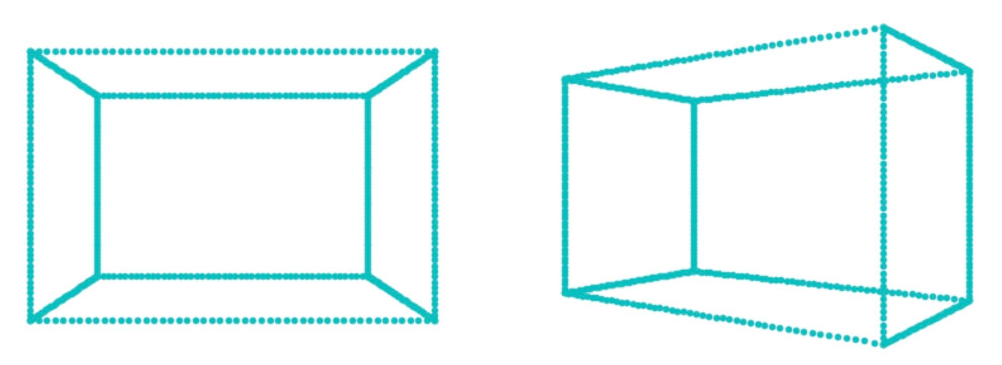
The projections of the cuboid as seen from the two cameras are shown below.

Find the fundamental matrix using the following OpenCV function:

F, mask = cv.findFundamentalMat(pts1, pts2, cv.FM_8POINT)

Since the intrinsic parameters matrix $K$ is the identity matrix, we have $E = F$. The essential matrix $E$ encodes the rotation and translation of the second camera relative to the first. To recover the pose of the second camera, use the following function:

_, rotation, translation, mask= cv.recoverPose(E, pts1, pts2)

The recovered projection matrix of the second camera is

M2_recovered = np.hstack((rotation, translation))

To recover the 3D points from their projections onto the left and right image planes, we use an optimization approach that minimizes the reconstruction error. Given the projected points in both cameras and their respective projection matrices, we aim to find the 3D points that best align with the observed 2D points in each view.

The reconstruction error measures the discrepancy between the actual projected 2D points and the re-projections of the estimated 3D points in both camera views. For each point, this error is calculated as the distance between the observed 2D points and their projections from the estimated 3D coordinates.

The total reconstruction error across all points can be expressed as the sum of individual errors from both views:

$$\text{Total Reconstruction Error} = \sum_i \left( \| x_L^i - M_L X_i \| + \| x^i_R - M_R X_i \| \right)$$

In this equation:

• $x_L^i$ and $x_R^i$ are the observed 2D points in the left and right images, respectively.
• $X_i$ is the estimated 3D point.
• $M_L$ and $M_R$ are the projection matrices for the left and right cameras.

By minimizing this total reconstruction error, we obtain a set of 3D points $\{ X_i \}$ that best align with the observed 2D image points $\{ x_L^i, x_R^i \}$ when projected back onto each camera's image plane. This optimization provides an effective method for reconstructing the 3D structure from multiple camera views.

In OpenCV we can use the function triangulatePoints to recover the 3D points:

X = cv.triangulatePoints(M1, M2_recovered, pts1.T, pts2.T)
X = X[:3] / X[3]  
X = X.T

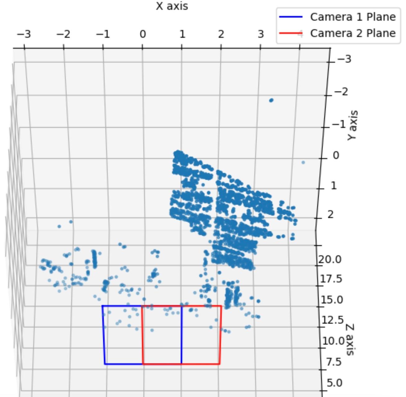
Structure From Motion (images)

Let’s revisit the process we discussed, but this time, using real left and right images to recover the 3D structure. We’ll follow these steps:

1. Detect features in both images. see Feature detectors and descriptors
2. Match features between the images using methods like feature matching and RANSAC.

3. Estimate the fundamental matrix to establish the relationship between the views.

F, mask = cv.findFundamentalMat(pts1, pts2, cv.RANSAC)

4. Compute the essential matrix from the fundamental matrix

E = K2.T @ F @ K1

5. Recover the camera pose (rotation and translation).

upts1 = cv.undistortPoints(pts1, K1, None).squeeze(1)
upts2 = cv.undistortPoints(pts2, K2, None).squeeze(1)
# Recover R, T withrespect to the first camera
_, R, T, mask = cv.recoverPose(E, upts1, upts2)

6. Define the projection matrices for both cameras.

M1 = K1 @ np.hstack((np.eye(3), np.zeros((3, 1))))
# Projection matrix for the second camera K2[R|T]
M2 = K2 @ np.hstack((R, T))

7. Triangulate the matched points to reconstruct the 3D structure.

X = cv.triangulatePoints(M1, M2, pts1[mask.ravel()==255].T, pts2[mask.ravel()==255].T)

# Convert from homogeneous coordinates to 3D
X = X[:3] / X[3]
pts_3d = X.T

Plot the 3D points

# Set up the 3D plot
fig = plt.figure()
ax = fig.add_subplot(111, projection='3d')
# Plot the camera plane
plot_camera_plane(ax, np.eye(3), np.array([0, 0, 0]), scale=1, color='blue', label='Camera 1')
plot_camera_plane(ax, R.T, -R.T@T, scale=1, color='red', label='Camera 2')
ax.scatter(pts_3d[:,0], pts_3d[:,1], pts_3d[:,2], marker='.')
# Label axes and set plot limits
ax.set_xlabel("X axis"), ax.set_ylabel("Y axis"), ax.set_zlabel("Z axis")
ax.legend()

ax.view_init(elev=-75, azim=-90)
plt.show()

Conclusion

In conclusion, our ability to perceive depth is thanks to our two eyes, each capturing a slightly different perspective of the world. By examining how objects in these two perspectives differ, we can calculate depth, a principle that applies similarly in computer vision. The pinhole camera model gave us a foundation to understand how cameras capture images and how intrinsic and extrinsic parameters influence image formation.

From there, we explored epipolar geometry, a framework essential for interpreting depth and relative positions of objects across two camera views. We learned how the Essential and Fundamental matrices mathematically capture the relationships between points in two images. These matrices allow us to extract information about camera movement and position relative to each other, crucial for applications such as 3D reconstruction and depth estimation.

By simulating a basic structure-from-motion example with a cuboid, we saw how two cameras positioned at different angles project the same 3D points into two different image planes. This experiment underscored the role of epipolar geometry in determining the relationship between points in different perspectives and how these relationships are key to depth perception.

Our understanding of these geometric principles forms the basis for advanced topics in 3D computer vision, like stereopsis and motion tracking, which leverage depth perception for a wide range of applications—from robotics to augmented reality. In future explorations, we'll build on these concepts to delve deeper into reconstructing 3D scenes from multiple views and exploring real-world applications.

FAQs

1. What is depth perception in computer vision?

   • Depth perception in computer vision refers to the ability of a system to perceive and estimate the distance of objects in a 3D environment based on visual input, typically using stereo vision, depth sensors, or multiple camera views.

2. How is depth estimated in computer vision?

   • Depth can be estimated using various techniques, such as stereo vision, structure-from-motion (SfM), and depth sensors like LiDAR. These methods analyze the disparity between images taken from different viewpoints or the geometry of the scene to calculate depth.

3. What is the role of stereo vision in depth estimation?

   • Stereo vision uses two or more cameras to capture images from different perspectives, and by comparing the disparity between corresponding points in the images, it calculates the depth information of the scene.

4. What is the fundamental matrix in computer vision?

   • The fundamental matrix is a key concept in stereo vision and epipolar geometry. It relates corresponding points between two images and is used to compute the epipolar lines, helping in the estimation of depth from stereo image pairs.

5. What is Structure-from-Motion (SfM)?

   • Structure-from-Motion (SfM) is a technique in computer vision that reconstructs the 3D structure of a scene from a series of 2D images. It uses the relative motion of the camera and corresponding points between images to generate 3D models.

6. How does epipolar geometry contribute to depth perception?

   • Epipolar geometry describes the geometric relationship between two views of the same scene. It simplifies depth estimation by reducing the search for corresponding points in stereo images to one-dimensional epipolar lines.

7. Can machine learning be used for depth estimation in computer vision?

   • Yes, machine learning, particularly deep learning, has become an essential tool in depth estimation. Convolutional neural networks (CNNs) and other neural networks can be trained to predict depth maps from single images or stereo pairs.

8. What are point clouds in 3D reconstruction?

   • Point clouds are sets of data points in 3D space, typically generated during 3D reconstruction processes. They represent the surface geometry of objects and environments, providing a detailed model of the scene.

9. How does camera calibration impact depth perception?

   • Camera calibration is critical for accurate depth perception. It involves determining the intrinsic and extrinsic parameters of the camera, ensuring that 3D space can be correctly mapped onto 2D images for precise depth estimation.

10. What are the challenges in depth perception for computer vision?

    • Some common challenges include handling occlusions (where objects block each other from view), ensuring accurate depth estimation in dynamic environments, managing noise and distortion in sensor data, and scaling the methods for real-time applications.