Feature Matching in Computer Vision: A Deep Dive into SIFT, NNDR, and RANSAC

In computer vision, feature detection and matching are essential tools for analyzing images. In the previous post, we explored feature detection and description. In this blog, we'll delve into feature matching, which enables us to match detected features across images and apply it to various applications such as image recognition and panoramic stitching. While deep learning techniques can accomplish these tasks, understanding traditional methods is crucial as it helps us grasp the underlying processes and enhance deep learning models.

Feature Extraction and Matching

Before matching two images, we begin with feature detection and description in each image. This involves identifying key points or regions that are distinctive and valuable for further analysis. In previous blog posts, we discussed detection of edges, corners and blobs. We also covered feature detection and description using SIFT

In this blog post, we'll explore how to use SIFT to describe features in two images and employ them for matching. We'll discuss the process of finding correspondences between images and applying it to various applications, such as recognition and panoramic stitching. Additionally, we'll provide OpenCV-Python code for implementation and discuss techniques for achieving robust correspondences.

Hover over each step:

Step 1: Detection

Step 2: Description

Step 3: Matching

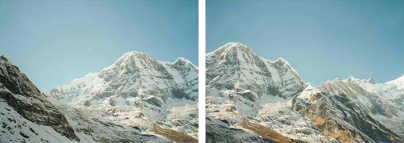
Image Source: Darya Frolova, Denis Simakov

Feature Matching

Suppose we have a feature, $f^1$ , in one image that we want to match to a feature in another image. To do this, we compute the distance between $f^1$ and all the features in the second image. When using SIFT, the feature descriptor has a length of $n=128$ . The feature with the smallest distance to $f^1$ is considered the best match. Given two feature vectors $f^1$ and $f^2$ the distance between the two vectors can be computed using:

\text{Sum of squared distance (SSD)} = \sum_{i=1}^{n} \left(f_{i}^{1} - f_{i}^{2}\right)^{2}

This formula sums the squared differences between corresponding elements of the two vectors, providing a measure of similarity between them. The lower the SSD, the more similar the feature descriptors are, indicating a potential match.

Problem with SSD

While Sum of Squared Differences (SSD) is effective for matching features, it has a limitation: non-distinctive features can produce multiple close matches. This means that even though a feature might have a low SSD with several features in another image, only one of these matches is likely to be correct. As a result, relying solely on SSD can lead to incorrect matches, especially in cases where the features aren't unique or distinctive enough.

The red feature is matched with three features in the right image, all of which have very similar distances. When a feature lacks distinctiveness, it can result in multiple close matches, making accurate matching difficult. In contrast, the green feature is matched with two features, but because it is more distinctive, the distance to the next best match is significantly higher.

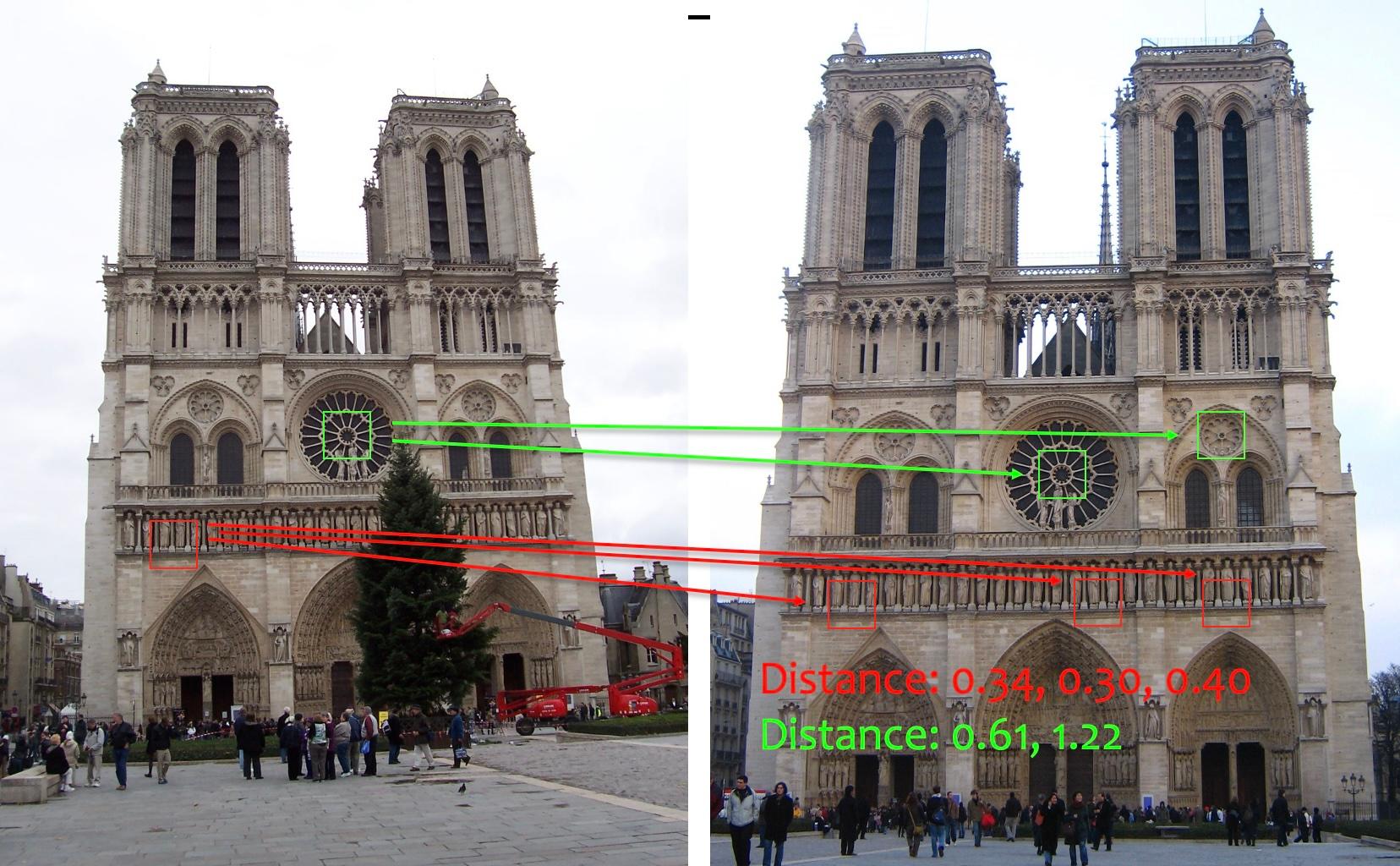
The red feature matches with multiple nearby features, showing low distinctiveness, while the green features higher distinctiveness results in a clear separation from other matches. Image Source: Wikipedia

Nearest Neighborhood Distance Ratio

The Nearest Neighbor Distance Ratio (NNDR) is a technique used in feature matching, evaluating the quality of matches by comparing the distance to the nearest neighbor with that of the second-nearest neighbor. This ratio acts as a robust filter, allowing for the identification of distinctive matches while mitigating ambiguity in the matching process.

NNDR = \frac{NN1}{NN2}

where $NN1$ is the distance to the first nearest neighbor and $NN2$ is the distance to the second nearest neighbor.

For the example above, the NNDR for the red matches is 0.30/0.34 = 0.88 while for the green match is 0.61/1.22 = 0.5. A higher NNDR indicates greater confidence in the quality of the match.

The following Python code performs feature matching between two images using the SIFT algorithm in OpenCV. It begins by loading the images and then uses SIFT to detect keypoints and compute their descriptors. A brute-force matcher (BFMatcher) is then employed to find the best matches between the descriptors of the two images. To ensure accurate matches, a Nearest Neighbor Distance Ratio (NNDR) test filters out less reliable matches. Finally, the good matches are visualized.

# Load images
image1 = cv2.imread('<Image 1>', cv2.IMREAD_GRAYSCALE)
image2 = cv2.imread('<Image 2>', cv2.IMREAD_GRAYSCALE)

# Initialize SIFT detector
feat = cv2.SIFT_create()

# Find the keypoints and descriptors with SIFT
keypoints1, descriptors1 = feat.detectAndCompute(image1, None)
keypoints2, descriptors2 = feat.detectAndCompute(image2, None)

# Create BFMatcher (Brute Force Matcher)
bf = cv2.BFMatcher()

# Match descriptors
matches = bf.knnMatch(descriptors1, descriptors2, k=2)

# Apply NN distance ratio test
good = []
for m,n in matches:
    if m.distance < 0.75*n.distance:
        good.append(m)
        
# Draw matches
img_matches = cv2.drawMatches(image1, keypoints1, image2, keypoints2, good[:50], cv2.DRAW_MATCHES_FLAGS_DRAW_RICH_KEYPOINTS, singlePointColor=(255, 0, 0), matchColor=(0, 255, 0))

# Plot the matches using Matplotlib
plt.figure(figsize=(14,8))
plt.imshow(img_matches)
plt.axis('off'), plt.tight_layout() 
plt.show()

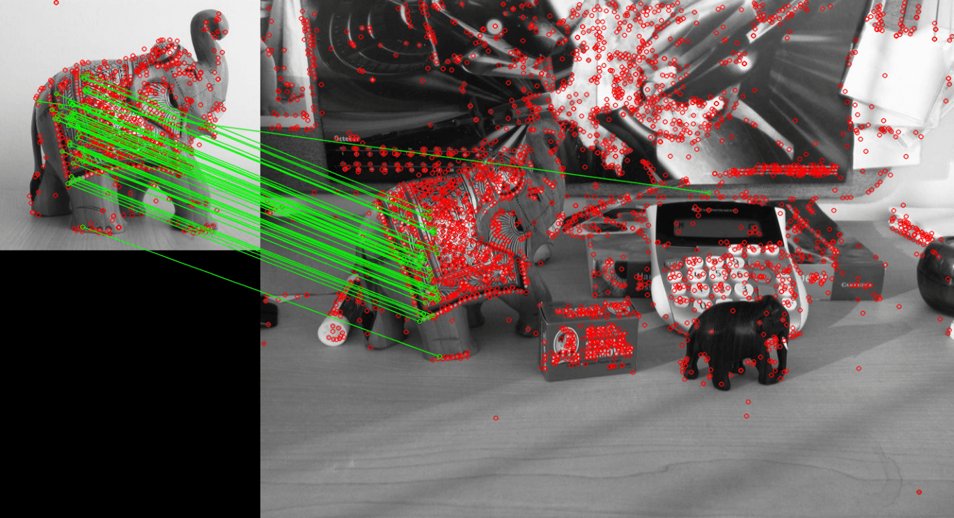
Visualization of feature matching between two images using SIFT. Red dots represent detected features, while the green lines highlight the top 50 matches identified through the NNDR test.

Model Fitting and Alignment

While NNDR improves match accuracy, incorrect matches can still slip through. To establish reliable correspondences between keypoints in two images, it's important to address unmatched points and incorrect matches. The solution lies in model fitting and alignment.

To illustrate this concept, let's consider an example with two transformed images that need to be matched. We can use SIFT to identify keypoints in each image and then measure the distance between these points, applying the NNDR test to filter out weaker matches. However, even with NNDR, some incorrect matches are inevitable.

Relying solely on the distance metric between descriptors can lead to some incorrect matches.

If we knew the correct transformation between the two images, we could align them and verify whether the keypoints correspond accurately by checking for overlap, easily discarding incorrect matches. However, this presents a "chicken and egg" problem—we need the correct matches to determine the transformation that aligns the images, but we also need the transformation to identify those correct matches. In the next section, we will explore RANSAC an algorithm that addresses this challenge.

Image Transformations

Before diving into RANSAC, it is important to understand image transformations and how they affect an image. An image transformation applies a set of rules, or a matrix, to all points in the image, changing their coordinates. These transformations can be described by a few key parameters and can be broadly classified into two categories: affine and projective transformations.

Affine Transformations

Affine transformations include translation, scaling, rotation, and shear. They can be represented by a matrix $T$ that linearly transforms the coordinates of points in an image. The transformation matrix for affine transformations is generally a $2 \times 3$ matrix that includes the parameters for scaling, rotation, and translation:

A = \begin{bmatrix} a & b & t_x \\ c & d & t_y \end{bmatrix}

Applying this transformation matrix $T$ to a point $(x, y)$ gives us the new coordinates $(x', y')$ :

\begin{bmatrix} x' \\ y' \end{bmatrix} = \begin{bmatrix} a & b & t_x \\ c & d & t_y \end{bmatrix} \begin{bmatrix} x \\ y \\ 1 \end{bmatrix}

Properties of Affine Transformations:

Lines map to lines.
Parallel lines remain parallel.
Ratios of distances between points are preserved.
They are closed under composition, meaning multiple affine transformations can be combined into a single transformation.

Projective Transformations (Homography)

Projective transformations, also known as perspective transformations or homographies, are more general and include affine transformations as well as projective warps. These transformations occur when viewing a three-dimensional scene from a two-dimensional plane and are represented by a $3 \times 3$ matrix:

H = \begin{bmatrix} h_{11} & h_{12} & h_{13} \\ h_{21} & h_{22} & h_{23} \\ h_{31} & h_{32} & h_{33} \end{bmatrix}

When applying this matrix to a point $(x, y)$ , we get new coordinates $(x', y')$ as follows:

\begin{bmatrix} x' \\ y' \\ w \end{bmatrix} = \begin{bmatrix} h_{11} & h_{12} & h_{13} \\ h_{21} & h_{22} & h_{23} \\ h_{31} & h_{32} & h_{33} \end{bmatrix} \begin{bmatrix} x \\ y \\ 1 \end{bmatrix}

To get the final coordinates, you normalize by dividing by ( w ):

x' = \frac{x'}{w}, \quad y' = \frac{y'}{w}

Properties of Projective Transformations:

Lines map to lines.
Parallel lines do not necessarily remain parallel.
Ratios of distances between points are not preserved.
They are also closed under composition.
The projective matrix is defined up to a scale factor and has 8 degrees of freedom.

Projective transformations are particularly useful for modeling the relationship between two images taken from different perspectives, as they can represent how one plane maps onto another.

To determine the Affine or Homography matrix, we need corresponding points from the two images. The Affine transformation has 6 degrees of freedom (DOF), requiring 3 points to provide the necessary 6 equations. Similarly, the Homography matrix, with its higher DOF, also relies on matching points to solve for the transformation.

Name	Matrix	# D.O.F.
Affine	$[A]$	6
Projective	$[H]$	8

RANdom SAmple Consensus (RANSAC)

RANSAC (Random Sample Consensus) is a robust algorithm used to estimate transformations between images, such as homography matrices, even when there are many incorrect matches between the images. Here is how RANSAC operates:

Random Sampling: The process starts by randomly selecting a small subset of matched points. For estimating a homography matrix, you need at least 4 such point pairs.
Model Estimation: With these randomly chosen points, RANSAC estimates the transformation model, whether it be a homography or affine matrix.
Consensus Evaluation: The algorithm then assesses how well this estimated model aligns with the remaining matched points. It applies the transformation and checks if other points fit within a specified tolerance. Points that conform well to the model are termed "inliers."
Iteration: Steps 1 through 3 are repeated numerous times, each time with a different random subset of points. Each iteration yields a different transformation model.
Best Model Selection: After many iterations, RANSAC identifies the model with the highest number of inliers. This model is considered the most accurate estimate of the transformation, as it aligns the images correctly and helps filter out incorrect matches.

By iteratively refining the transformation model through random sampling, RANSAC effectively handles scenarios with numerous incorrect correspondences. It provides a reliable method for determining the correct image alignment, even under challenging conditions.

The following OpenCV function can be used to find the Homography matrix using demonstrates how RANSAC is used to compute the homography matrix. During this process, it also identifies the correct matches (inliers) between the images.

# Extract the corresponding set of matched keypoints
src_pts = np.float32([ keypoints1[m.queryIdx].pt for m in good ]).reshape(-1,1,2)
dst_pts = np.float32([ keypoints2[m.trainIdx].pt for m in good ]).reshape(-1,1,2)

# Use RANSAC to estimate the homography matrix. mask contains the list of inliers
H, mask = cv2.findHomography(src_pts, dst_pts, cv2.RANSAC, ransacReprojThreshold=5)

# Draw the matched keypoints
output_image = cv2.drawMatches(image1,keypoints1,image2,keypoints2,good, cv.DRAW_MATCHES_FLAGS_DRAW_RICH_KEYPOINTS, matchesMask=mask.ravel().tolist())

Finding Correct Matches Between Two Images Using a Homography Matrix

Applications

Image Stitching

Image stitching is a computer vision technique that seamlessly merges multiple overlapping images into a single, larger panoramic view. This process involves aligning and blending the images based on key points and features. By applying transformations such as affine and projective, we can achieve precise alignment. Specifically, the homography matrix is used to transform and align the images accurately. The following image illustrates the alignment achieved using the homography matrix.

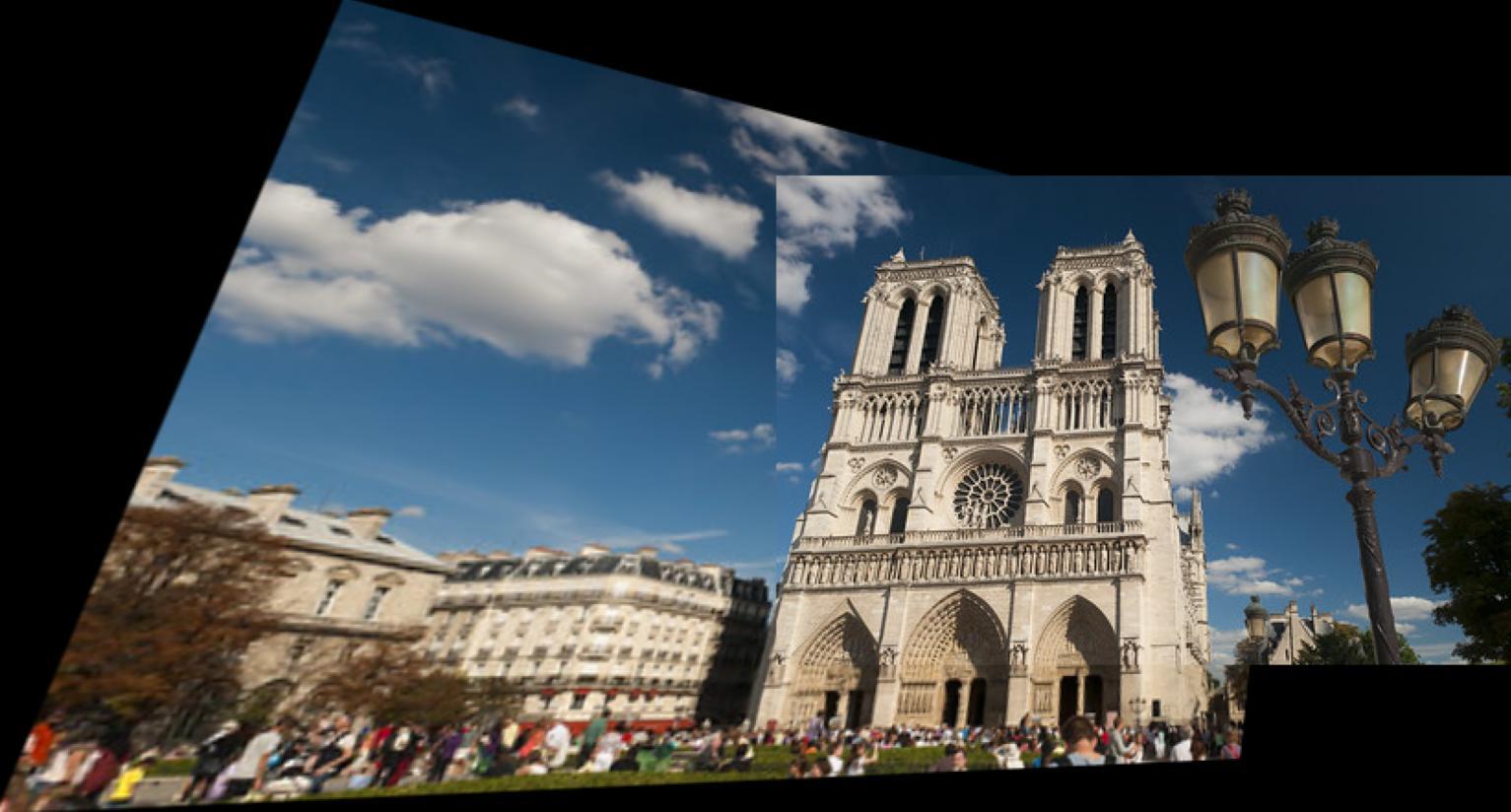
Object Recognition

The homography matrix can be used in object recognition to establish a relationship between two different views of the same object. By mapping points from one image to corresponding points in another, the homography matrix enables the transformation of an object's appearance across different perspectives. This is particularly useful in recognizing objects that are captured from varying angles or distances. By applying the homography matrix, the image can be warped or aligned to match a reference image.

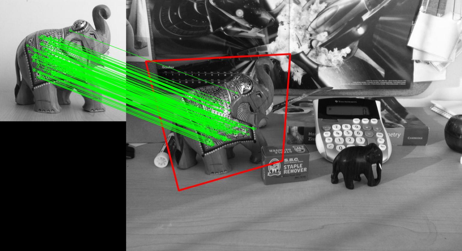
Homography matrix computed from corresponding keypoints is used to align the image for object recognition

Related Posts

Test Your Knowledge

1/10

What is the primary purpose of feature matching in computer vision?